 Have you ever been working on a project in Excel just to realize that it would look better if it were arranged horizontally instead of vertically (swapping around the Rows and Columns)? Here is an age old Excel trick that works whether you’re using Excel 2010, 2007, 2003, or even the stone age Excel 2000. (Gasp!)
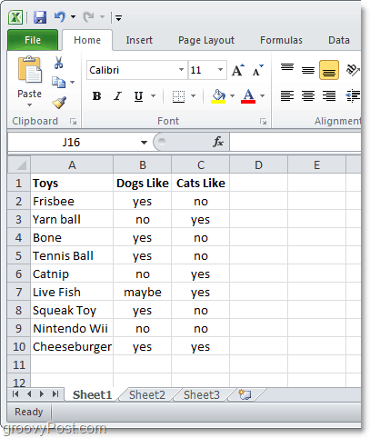
Here we have a typical spreadsheet in Excel 2010 that is lined up vertically using a column style. Just for demonstration sake, we’re going to go ahead and change this into a horizontal row style.
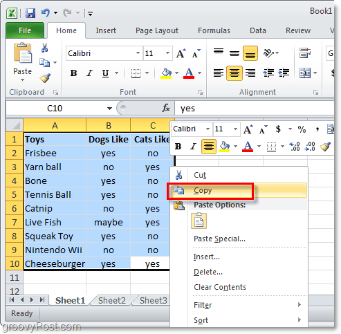
1. In Excel 2010, Select all of the cells that you want to convert. Once you’ve Selected them, Right-Click and Click Copy.*
*You can also use the keyboard shortcut Ctrl+C to copy.
2. Now Right-Click and empty cell and Select Paste Options: > Transpose. One of the groovy features in Outlook 2010 is that it will even show you a preview of what the paste will look like before it happens.
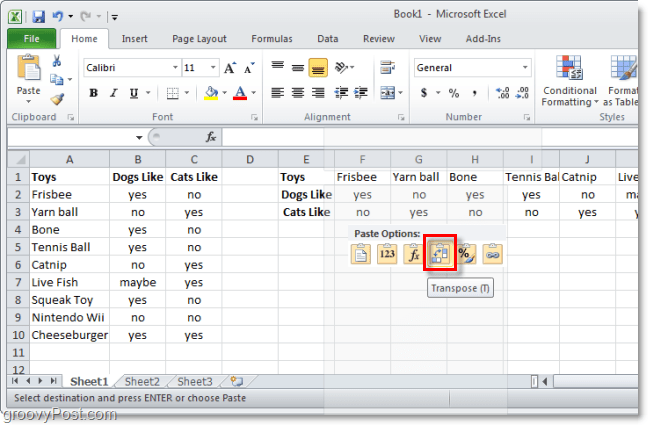
2.b Alternatively if the Paste Options aren’t showing up. Right-Click an empty cell and Select Paste Special.

3. From the Paste Special window Check the Transpose box and then Click OK.

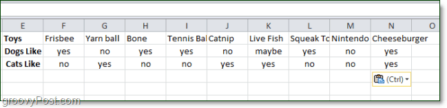
The result will be that your data has been converted (transposed) to a new layout style. This tip will work the opposite way as well if you ever need to convert your horizontal row data sheets into the vertical column style.


Clint
March 30, 2011 at 12:37 pm
I can’t seem to get the transpose option when copying from one excel file and pasting to another. I have to add the extra steps of copying as-is, copy THAT list, transpose it to where I need it, then delete the original list I copied over. There’s got to be something I’m missing.
JC
February 29, 2012 at 12:22 pm
This is an old post, so I’m sure you’ve figured this out, but I just ran into this problem and you solved it for me. I had been using transpose for a week and suddenly I couldn’t anymore. In searching for an answer, your post made me realized I had opened a second Excel session and, as you pointed out, you can’t transpose from one session to another. However, you can open up a second file in your current session and successfully transpose from one spreadsheet to the other, which is what I had been doing previously. They really should fix this, since sometimes you want to have two sessions open to see full pages side by side when copying and pasting. Anyway, thanks for solving my little mystery!
Mary Anne Sullivan
January 16, 2013 at 11:46 am
I’m very glad you posted this b/c i couldn’t figure out what i was doing wrong!
VLad
October 25, 2011 at 8:00 pm
Thanks for help Austin Krause!
Excellent easy to read and straightforward article! Five Stars!
Wendy Lauber Kilbourne
August 13, 2012 at 8:46 am
SWEET! 5 STARS!!
Steve Krause
August 13, 2012 at 9:32 am
Hi Wendy — welcome to my blog. I’m glad the tip helped you out!
Have you tried out Excel 2013 yet? What do you think of it so far?
Shah
April 6, 2013 at 3:54 am
Hi Steve,
Very nice feature, I am using this from 2010. Easy me to use in 2013.
Dennis Mungle
December 17, 2012 at 8:02 am
Thanks. Too easy, I just forgot the steps.
Phil Olivero
April 25, 2013 at 6:56 am
Perfect instructions, pictures replace a thousand words. The feature saved me a lot of time. I will use your Blog going forward.
Lesley Payne
September 6, 2013 at 2:43 am
Hi, Many thanks, such a big help. Its something I have struggled with and once you know the answer you think, DOH! why didn’t I do that before. :)
ankruxandra
October 15, 2013 at 8:53 am
Thank you!! Great help for me!!!
Kate
October 25, 2013 at 1:55 am
Wonderful thank you,was given an assignment at work .Managed to do it quickly with your help.
Ed
April 14, 2014 at 3:41 pm
In your example, if the ‘Cats Like’ column referred to a different tab on the same workbook, is there a way to make this work when transposing columns to rows or vice versa? If so, please explain. I can only get the table to work if all the value come from the same tab.
Thanks,
John
December 13, 2017 at 9:51 am
While this function works with cells containing manually input data, it doesn’t seem to work with cells containing formulas. When I try to convert cells containing formulas or cells linked to other worksheet pages, the horizontal to vertical converted cell display reads “#REF!”.
Any ideas?