Microsoft Excel: How To Alternate the Color Between Rows

Sometimes you need to make large spreadsheets easier to read. Alternating colors between rows is an excellent way to do it. Here’s how.
Sometimes you need to make large spreadsheets easier to read. Alternating colors between rows is an excellent way to do it. Here’s how.
Alternate Color Between Excel Rows
In Excel, assigning an alternating color scheme to rows is known as color banding.
Start by selecting the cells you want to apply color banding too. Or press Ctrl+A to select the entire sheet.


Next, select the Home tab on the Ribbon, select Styles, and click Conditional Formatting.


A drop-down menu will display; click New Rule.


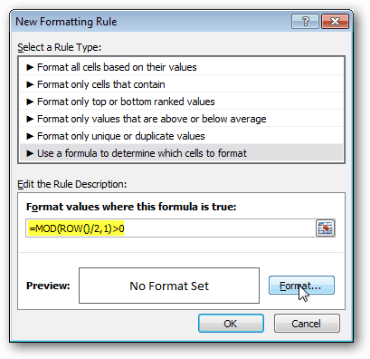
The New Formatting Rule dialog appears. Click the bottom option labeled Use a Formula to Determine Which Cells to Format.
In the empty format value field, copy and paste in the following formula:
=MOD(ROW()/2,1)>0The New Formatting Rule window will look like this. Click Format.


Pick a fill color and click OK.


The New Formatting Rule windows will display the color Preview. Click OK.


The section of your spreadsheet will now be color-banded.


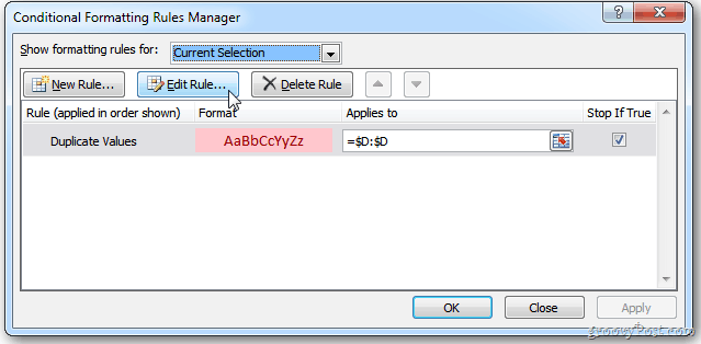
If you want to change the color or add more cells, highlight the cells on the spreadsheet. Then on the Ribbon, go to Conditional Formatting > > Manage Rules.


The Conditional Formatting Rules Manager window comes up. Click Edit Rule.


The Edit Formatting Screen appears and can adjust accordingly.


15 Comments
Leave a Reply
Leave a Reply


Dave
October 18, 2011 at 5:32 am
There is an obvious typo in two places where the number 9 is inserted in place of the left parent (shift 9). Who hasn’t done that!
I question the formula. Use =mod(row()/2)>0. It works equally well and is less convoluted.
ChuckZilla
October 18, 2011 at 9:23 pm
I used your formula and it didn’t work.
Dave
October 18, 2011 at 12:02 pm
Oops, should be =mod(row(),2)>0
Peter Devos
October 22, 2011 at 7:44 am
both formulas
=mod(row(),2)>0
=mod(row()/2,1)>0
are giving error message in MS office Pro 2010 ?????
James M Singleton
October 20, 2011 at 11:13 am
I have been looking for a Windows application to automatically do it like an Excel addon.
Michael
October 22, 2011 at 4:36 am
Why not use the Format as Table button beside it to do it automaticaly, then turn the header off and select your banding style on the Design tab that appears?
Avinash Arora
October 31, 2011 at 10:43 am
I was thinking the same thing…there are much easier ways to do this, however conditional formatting is an amazing tool everyone using excel for presentation data should learn. Makes accounting and notable figures much more easy to find and work with.
Peter Devos
October 22, 2011 at 7:52 am
Here is the correct formula ( separator is instead of )!
=MOD(ROW()/2;1)>0
nury
October 24, 2011 at 4:59 am
thank you i just tried it and it worked thanx again
Steve Krause
October 24, 2011 at 3:15 pm
NP Nury – it’s a great trick I agree.
Free Unlimited Internet
October 29, 2011 at 4:42 am
This really helped me a lot. I struggled with this for 1 hr could you be leave it.
Techno Sage
November 5, 2011 at 9:52 pm
Very nice tip!
don
January 30, 2012 at 6:32 pm
way too complex, =iseven(row()) or =isodd(row())
does the same thing
Scott
May 11, 2012 at 2:20 pm
Prior to XL2007, ISEVEN and ISODD required loading the Analysis Toolpak.
In the mod formula, the >0 part isn’t necessary. 0 will evaluate to FALSE and any non-zero number will evaluate to TRUE, therefore;
=MOD(ROW(),2)
will suffice.
If you want to start with a blank row, instead of a filled row, just subtract 1 in the formula:
=MOD(ROW(),2)-1
laune
October 29, 2014 at 8:41 am
if error occurs
should be a “;” instead of a “,” in the formula between row() & 2….
so. =mod(row();2)=0